import matplotlib.pyplot as plt
plt.figure()
plt.plot([1, 2, 3], [4, 5, 6])
plt.title("Sales")
plt.xlabel("Quarter")
plt.show()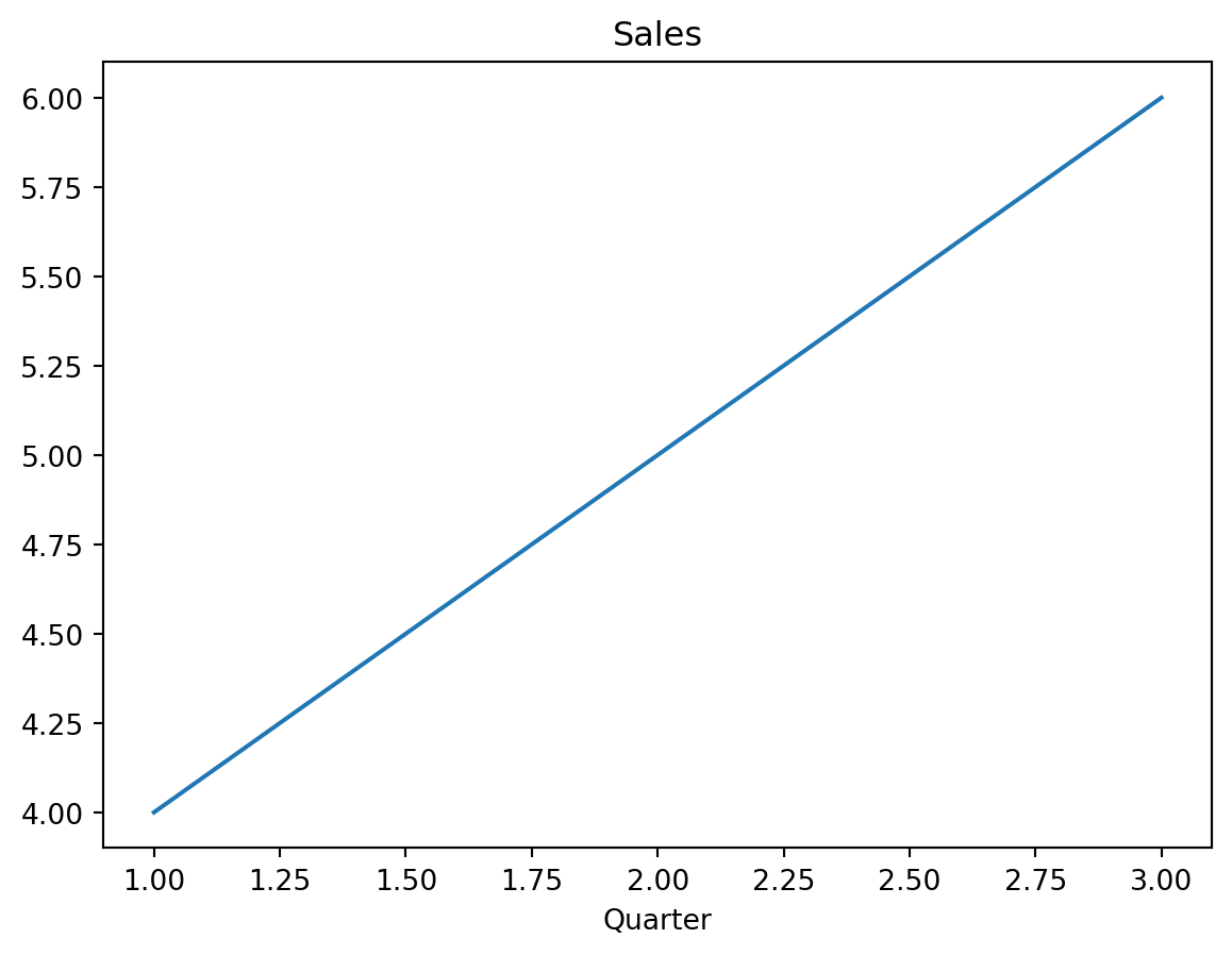
This module is mostly conceptual. The goal is to make fig, ax = plt.subplots() feel concrete: what objects are created, how they relate to each other, and why the object-oriented API is the default habit to build.
Every matplotlib plot is built from three nested concepts. Internalizing this hierarchy explains much of how matplotlib works.
┌─────────────────────────────────────────────────────┐
│ FIGURE: the window / page / canvas                  │
│                                                     │
│   ┌──────────────────┐     ┌──────────────────┐     │
│   │ AXES             │     │ AXES             │     │
│   │ one plot panel   │     │ one plot panel   │     │
│   │                  │     │                  │     │
│   │   ┌─ title ─┐    │     │   ┌─ title ─┐    │     │
│   │   │ • •     │    │     │   │ • •     │    │     │
│   │   │ • • •   │    │     │   │ • • •   │    │     │
│   │   └─x-axis──┘    │     │   └─x-axis──┘    │     │
│   │      y-axis      │     │      y-axis      │     │
│   └──────────────────┘     └──────────────────┘     │
│                                                     │
│ ARTISTS: lines, dots, text, legends, ticks, patches │
└─────────────────────────────────────────────────────┘
There are three terms to keep straight:
Figure per image saved or displayed. Think of it as the sheet of paper.Artist objects.A Figure can contain many Axes objects. Each Axes usually contains two Axis objects: the x-axis and y-axis rulers.
| ggplot2 concept | matplotlib concept |
|---|---|
| the whole rendered plot | Figure |
| one facet panel | Axes |
geom_point() output |
an Artist, often a PathCollection |
geom_line() output |
an Artist, usually a Line2D |
| theme text element | an Artist, usually a Text object |
In ggplot2, these objects are mostly hidden behind the grammar of graphics. In matplotlib, the objects are explicit and are modified through method calls. That is the main imperative shift.
Matplotlib has two common ways to draw the same plot. Many tutorials mix them freely, which is one reason matplotlib can feel confusing at first.
The pyplot API is MATLAB-style. It keeps a hidden global idea of the current figure and current axes. Each plt.* call modifies whichever object is currently active.
import matplotlib.pyplot as plt

plt.figure()
plt.plot([1, 2, 3], [4, 5, 6])
plt.title("Sales")
plt.xlabel("Quarter")
plt.show()
This is convenient for quick one-off plots, but it becomes ambiguous when there are multiple panels. If there are several axes, plt.title() titles whichever axes matplotlib considers current.
The object-oriented API creates explicit Figure and Axes objects, then calls methods on those objects.
import matplotlib.pyplot as plt

fig, ax = plt.subplots()  # explicitly create Figure and Axes
ax.plot([1, 2, 3], [4, 5, 6])  # draw on this Axes object
ax.set_title("Sales")
ax.set_xlabel("Quarter")
plt.show()
With the object-oriented API, every modification targets a specific object. There is no need to depend on hidden global state.
pyplot style                         OO style
──────────────────────               ───────────────────────
plt → hidden state → drawing          you → fig, ax → drawing
The standard idiom is a small hybrid: plt.subplots() is a pyplot function, but it returns explicit Figure and Axes objects so the rest of the code can use the OO API.
Use the object-oriented API for anything beyond a throwaway exploratory plot.
The advantages become obvious as soon as a figure has more than one subplot. With pyplot, plt.title() depends on which panel is current. With the OO API, ax1.set_title(...) and ax2.set_title(...) are explicit.
The OO style is also easier to:
ax as an argumentPyplot is still fine for a quick plt.hist(data) in an exploratory notebook cell. For reusable notes, teaching material, and publication figures, the OO API should be the default.
This book uses a local uv environment. The project dependencies include matplotlib, NumPy, pandas, seaborn, SciPy, Jupyter Notebook, and IPython kernel support.
From the project root:
uv sync
uv run jupyter notebook
The first code cell of most plotting notebooks usually starts with:
import matplotlib.pyplot as plt
import numpy as np
No backend configuration is required for normal notebook use. VS Code’s Jupyter integration and Jupyter Notebook render plots inline by default.
A backend is the rendering engine that turns matplotlib instructions into pixels or vector graphics. It is rarely necessary to set the backend manually, but the categories are useful when debugging.
┌──────────────────────────────────────────────────────┐
│ Interactive backends: open a window                  │
│ • MacOSX — common on macOS for plain Python          │
│ • QtAgg / Qt5Agg — cross-platform GUI                │
│ • TkAgg — Tk-based GUI fallback                      │
├──────────────────────────────────────────────────────┤
│ Inline backends: embed in notebooks                  │
│ • inline — static PNG in the notebook                │
│ • widget — interactive zoom/pan in the notebook      │
├──────────────────────────────────────────────────────┤
│ Non-interactive / file-only backends                 │
│ • Agg — PNG output, no display, useful in scripts    │
│ • PDF, SVG, PS — vector formats for publication      │
└──────────────────────────────────────────────────────┘
In a notebook, the inline backend is usually enough. For interactive zoom and pan inside notebooks, %matplotlib widget can be used after installing ipympl. For now, the default inline behavior is the cleanest baseline.
This is the minimal plot that demonstrates the standard matplotlib workflow.
import matplotlib.pyplot as plt
import numpy as np

x = np.linspace(0, 10, 100)
y = np.sin(x)

fig, ax = plt.subplots()
ax.plot(x, y)
ax.set_title("My first OO-API plot")
ax.set_xlabel("x")
ax.set_ylabel("sin(x)")
plt.show()

print(type(fig))
print(type(ax))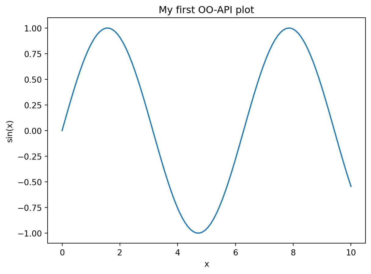
<class 'matplotlib.figure.Figure'>
<class 'matplotlib.axes._axes.Axes'>Figure is the full canvas.Axes is one plot panel inside a figure.Axis is a ruler-like component of an axes, such as the x-axis or y-axis.Artist is any visible object drawn on the figure.plt.subplots() is the standard entry point because it creates explicit Figure and Axes objects.