8  Module 7 — Styling and Themes

This module is the matplotlib counterpart to ggplot2’s theme() system and theme_*() functions.

The goal is to stop styling each plot individually and instead set defaults once. By the end, the direction is toward a reusable Radiology AI Unit style that automatically applies to every figure.

The core mental model:

┌─────────────────────────────────────────────────────────┐
│ rcParams = a giant dictionary of default settings.      │
│ Every matplotlib function reads from it.                │
│                                                         │
│ Change rcParams once → every subsequent plot reflects   │
│ the change. No more repeating yourself.                 │
└─────────────────────────────────────────────────────────┘

There are three layers of styling, in increasing order of permanence:

┌────────────────────────────────────────────────────────────┐
│ Layer 1: Per-plot keyword arguments                        │
│ ax.plot(x, y, color="red", linewidth=2)                   │
│ → applies only to this call                                │
├────────────────────────────────────────────────────────────┤
│ Layer 2: rcParams modification, session-wide               │
│ plt.rcParams["axes.titlesize"] = 14                       │
│ → applies to all plots in this Python session              │
├────────────────────────────────────────────────────────────┤
│ Layer 3: Style sheets / matplotlibrc files                 │
│ plt.style.use("my-style")                                 │
│ → reusable, version-controllable, shareable                │
└────────────────────────────────────────────────────────────┘

The previous modules mostly used Layer 1. This module moves upward.

8.1 1. rcParams: the central settings dictionary

rcParams, short for runtime configuration parameters, is a dictionary-like object with hundreds of settings.

import matplotlib.pyplot as plt
import matplotlib as mpl
import numpy as np

# Inspect a setting
print(plt.rcParams["figure.figsize"])
print(plt.rcParams["axes.titlesize"])

[7.0, 5.0]
large

The keys are dot-namespaced by what they affect, such as:

• figure.*
• axes.*
• xtick.*
• ytick.*
• legend.*
• font.*
• lines.*

Changing a setting affects future plots in the current Python session.

x = np.linspace(0, 10, 100)
y = np.sin(x)

with mpl.rc_context({
    "figure.figsize": (8, 5),
    "axes.titlesize": 14,
    "font.family": "sans-serif",
}):
    fig, ax = plt.subplots()
    ax.plot(x, y)
    ax.set_title("Plot using temporary rcParams")
    ax.set_xlabel("x")
    ax.set_ylabel("sin(x)")
    plt.show()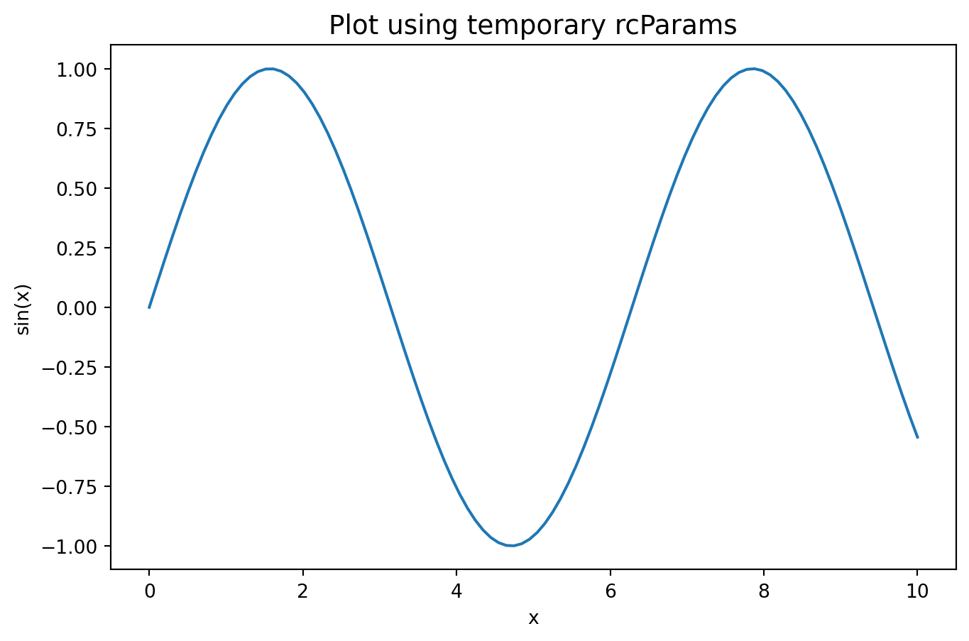

This example uses mpl.rc_context(...) so the settings are temporary and do not leak into the rest of the notebook. In normal project code, plt.rcParams[...] = ... or plt.rcParams.update(...) changes settings for all subsequent plots in the session.

A useful starter set:

radiology_style = {
    # Figure
    "figure.figsize": (8, 5),
    "figure.dpi": 100,
    "savefig.dpi": 300,
    "savefig.bbox": "tight",

    # Fonts
    "font.family": "sans-serif",
    "font.size": 11,
    "axes.titlesize": 13,
    "axes.labelsize": 11,
    "xtick.labelsize": 10,
    "ytick.labelsize": 10,
    "legend.fontsize": 10,

    # Axes appearance
    "axes.spines.top": False,
    "axes.spines.right": False,
    "axes.grid": True,
    "axes.grid.axis": "y",
    "grid.linestyle": ":",
    "grid.alpha": 0.5,

    # Lines and markers
    "lines.linewidth": 2.0,
    "lines.markersize": 6,
}

with mpl.rc_context(radiology_style):
    fig, ax = plt.subplots()
    ax.plot(x, y, marker="o", label="sin(x)")
    ax.set_title("Styled by rcParams")
    ax.set_xlabel("x")
    ax.set_ylabel("sin(x)")
    ax.legend()
    plt.show()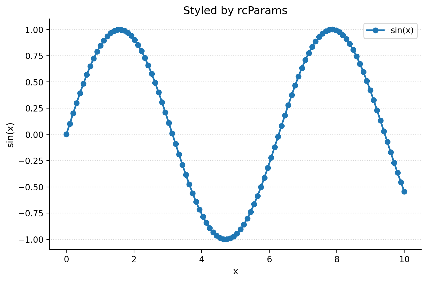

After these defaults are active, every new fig, ax = plt.subplots() inherits them. This removes repetitive boilerplate such as hiding the top and right spines or setting a light y-axis grid on every plot.

8.2 2. Discovering settings

There are two reliable discovery tools: search the keys and inspect the active matplotlibrc file.

# All rcParams keys that mention "tick"
tick_keys = [k for k in plt.rcParams if "tick" in k]
print(tick_keys[:20])
print(f"... {len(tick_keys)} tick-related keys total")

# Path to the active matplotlibrc reference file
print(mpl.matplotlib_fname())

['xtick.alignment', 'xtick.bottom', 'xtick.color', 'xtick.direction', 'xtick.labelbottom', 'xtick.labelcolor', 'xtick.labelsize', 'xtick.labeltop', 'xtick.major.bottom', 'xtick.major.pad', 'xtick.major.size', 'xtick.major.top', 'xtick.major.width', 'xtick.minor.bottom', 'xtick.minor.ndivs', 'xtick.minor.pad', 'xtick.minor.size', 'xtick.minor.top', 'xtick.minor.visible', 'xtick.minor.width']
... 42 tick-related keys total
/Users/kittipos/my_book/py-plot-notes/.venv/lib/python3.12/site-packages/matplotlib/mpl-data/matplotlibrc

To reset everything to factory defaults:

plt.rcdefaults()

The full list of defaults lives in a file called matplotlibrc inside the matplotlib installation. Treat it as a reference, not something to edit directly.

Useful rcParams categories:

figure.*        size, dpi, layout
axes.*          spines, titles, grid, prop_cycle (color cycle)
font.*          family, size, weight
xtick.*         label sizes, directions, lengths
ytick.*         label sizes, directions, lengths
legend.*        fontsize, frameon, loc
lines.*         linewidth, markersize, default style
savefig.*       dpi, bbox, format

8.3 3. The color cycle revisited

From Module 5, the default color cycle is set through axes.prop_cycle. To install a colorblind-safe palette globally, use cycler. In a notebook, it is safer to demonstrate this with a temporary context.

from cycler import cycler

okabe_ito = [
    "#000000", "#E69F00", "#56B4E9", "#009E73",
    "#F0E442", "#0072B2", "#D55E00", "#CC79A7",
]

with mpl.rc_context({"axes.prop_cycle": cycler(color=okabe_ito)}):
    fig, ax = plt.subplots(figsize=(7, 4))
    for i in range(5):
        ax.plot(x, np.sin(x) + i, label=f"line {i}")
    ax.legend(ncol=2)
    ax.set_title("Okabe-Ito color cycle")
    plt.show()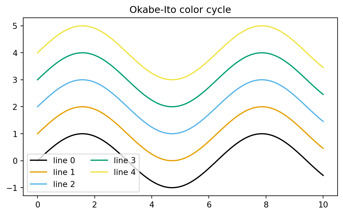

In a normal script or session, the persistent version would be:

plt.rcParams["axes.prop_cycle"] = cycler(color=okabe_ito)

Multiple properties can cycle together, such as color and linestyle. This is useful for grayscale-printable figures.

line_styles = ["-", "--", ":", "-.", "-", "--", ":", "-."]

with mpl.rc_context({"axes.prop_cycle": cycler(color=okabe_ito) + cycler(linestyle=line_styles)}):
    fig, ax = plt.subplots(figsize=(7, 4))
    for i in range(5):
        ax.plot(x, np.sin(x) + i, label=f"line {i}")
    ax.legend(ncol=2)
    ax.set_title("Cycling color and linestyle")
    plt.show()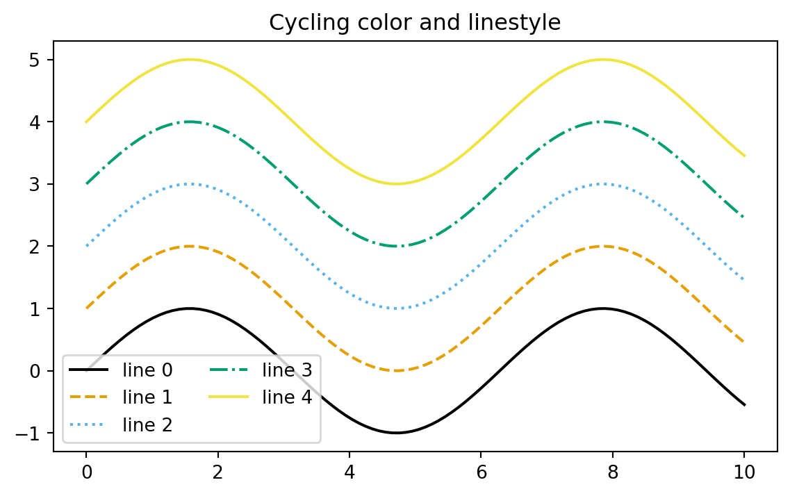

8.4 4. Style sheets: reusable presets

A style sheet is a saved bundle of rcParams that can be activated in one line. Matplotlib ships with many styles.

print(plt.style.available[:12])
print(f"... {len(plt.style.available)} styles available")

['Solarize_Light2', '_classic_test_patch', '_mpl-gallery', '_mpl-gallery-nogrid', 'bmh', 'classic', 'dark_background', 'fast', 'fivethirtyeight', 'ggplot', 'grayscale', 'petroff10']
... 29 styles available

Common examples include:

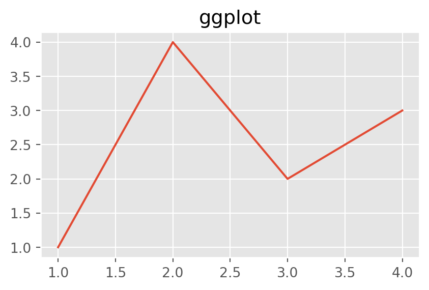
plt.style.use("ggplot")
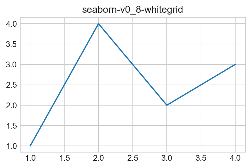
plt.style.use("seaborn-v0_8-whitegrid")
plt.style.use("default")

Use plt.style.context(...) for temporary styling that reverts after the with block.

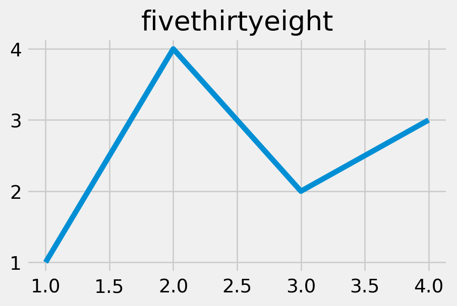
for style in ["default", "ggplot", "seaborn-v0_8-whitegrid", "fivethirtyeight"]:
    with plt.style.context(style):
        fig, ax = plt.subplots(figsize=(5, 3))
        ax.plot([1, 2, 3, 4], [1, 4, 2, 3])
        ax.set_title(style)
        plt.show()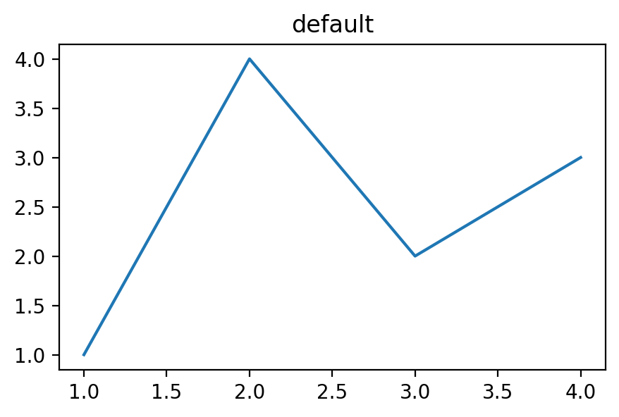

plt.style.use(...)      permanent for the session
plt.style.context(...)  temporary, scoped to a with block

8.5 5. Writing a custom style sheet

A style sheet is a plain text file with one key: value setting per line. For a project, a version-controlled style file is usually better than a per-user style because it travels with the repository.

Example styles/radai.mplstyle:

# Radiology AI Unit — publication style

figure.figsize: 8, 5
figure.dpi: 100
savefig.dpi: 300
savefig.bbox: tight

font.family: sans-serif
font.size: 11
axes.titlesize: 13
axes.titleweight: bold
axes.titlelocation: left
axes.labelsize: 11

axes.spines.top: False
axes.spines.right: False
axes.grid: True
axes.grid.axis: y
grid.linestyle: :
grid.alpha: 0.5
grid.color: gray

lines.linewidth: 2.0
lines.markersize: 6

xtick.direction: out
ytick.direction: out

legend.frameon: False
legend.fontsize: 10

axes.prop_cycle: cycler('color', ['000000', 'E69F00', '56B4E9', '009E73', 'F0E442', '0072B2', 'D55E00', 'CC79A7'])

Syntax notes:

• no quotes around strings
• comma separates figsize width and height
• colors inside prop_cycle omit #
• lines starting with # are comments

Where to put the style file:

Per-user:
~/.matplotlib/stylelib/myname.mplstyle
→ use as: plt.style.use("myname")

Per-project:
/your/project/styles/myname.mplstyle
→ use as: plt.style.use("/your/project/styles/myname.mplstyle")
→ version-controlled and reproducible

For a Quarto book or paper repository, the per-project approach is usually preferable.

The current book can demonstrate this by writing a small project-local style file under styles/.

from pathlib import Path

style_dir = Path("styles")
style_dir.mkdir(exist_ok=True)
style_path = style_dir / "radai.mplstyle"
style_path.write_text("""# Radiology AI Unit — publication style

figure.figsize: 8, 5
figure.dpi: 100
savefig.dpi: 300
savefig.bbox: tight

font.family: sans-serif
font.size: 11
axes.titlesize: 13
axes.titleweight: bold
axes.titlelocation: left
axes.labelsize: 11

axes.spines.top: False
axes.spines.right: False
axes.grid: True
axes.grid.axis: y
grid.linestyle: :
grid.alpha: 0.5
grid.color: gray

lines.linewidth: 2.0
lines.markersize: 6

xtick.direction: out
ytick.direction: out

legend.frameon: False
legend.fontsize: 10

axes.prop_cycle: cycler('color', ['000000', 'E69F00', '56B4E9', '009E73', 'F0E442', '0072B2', 'D55E00', 'CC79A7'])
""")
print(style_path)

styles/radai.mplstyle

with plt.style.context("styles/radai.mplstyle"):
    fig, ax = plt.subplots()
    ax.plot(x, np.sin(x), label="Sensitivity")
    ax.plot(x, np.cos(x), label="Specificity")
    ax.set_title("Diagnostic performance")
    ax.set_xlabel("Threshold")
    ax.set_ylabel("Performance")
    ax.legend()
    plt.show()

8.6 6. Combining styles

Style sheets can be stacked. Later styles override earlier ones:

plt.style.use(["seaborn-v0_8-whitegrid", "radai"])

This applies seaborn’s whitegrid first, then applies local overrides on top.

with plt.style.context(["seaborn-v0_8-whitegrid", "styles/radai.mplstyle"]):
    fig, ax = plt.subplots()
    ax.plot(x, np.sin(x), label="Sensitivity")
    ax.plot(x, np.cos(x), label="Specificity")
    ax.set_title("Stacked styles")
    ax.legend()
    plt.show()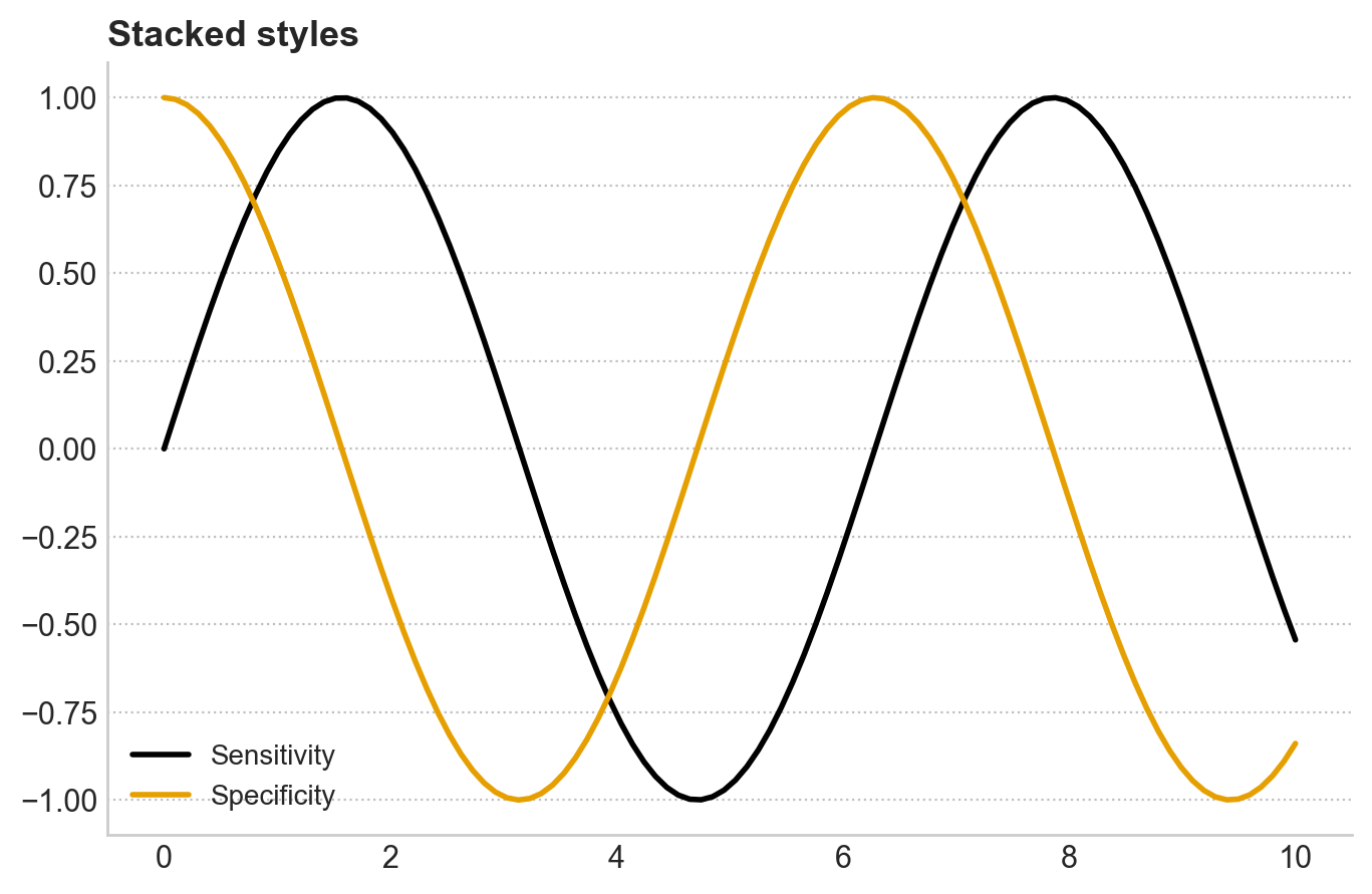

8.7 7. The with pattern for one-off styling

Sometimes one figure should look different, such as a slide figure needing larger fonts. Use a context manager.

with plt.rc_context({"font.size": 16, "axes.titlesize": 20, "lines.linewidth": 3}):
    fig, ax = plt.subplots(figsize=(10, 6))
    ax.plot(x, np.sin(x))
    ax.set_title("Big version for slides")
    ax.set_xlabel("x")
    ax.set_ylabel("sin(x)")
    plt.show()

# After the with block, settings return to normal.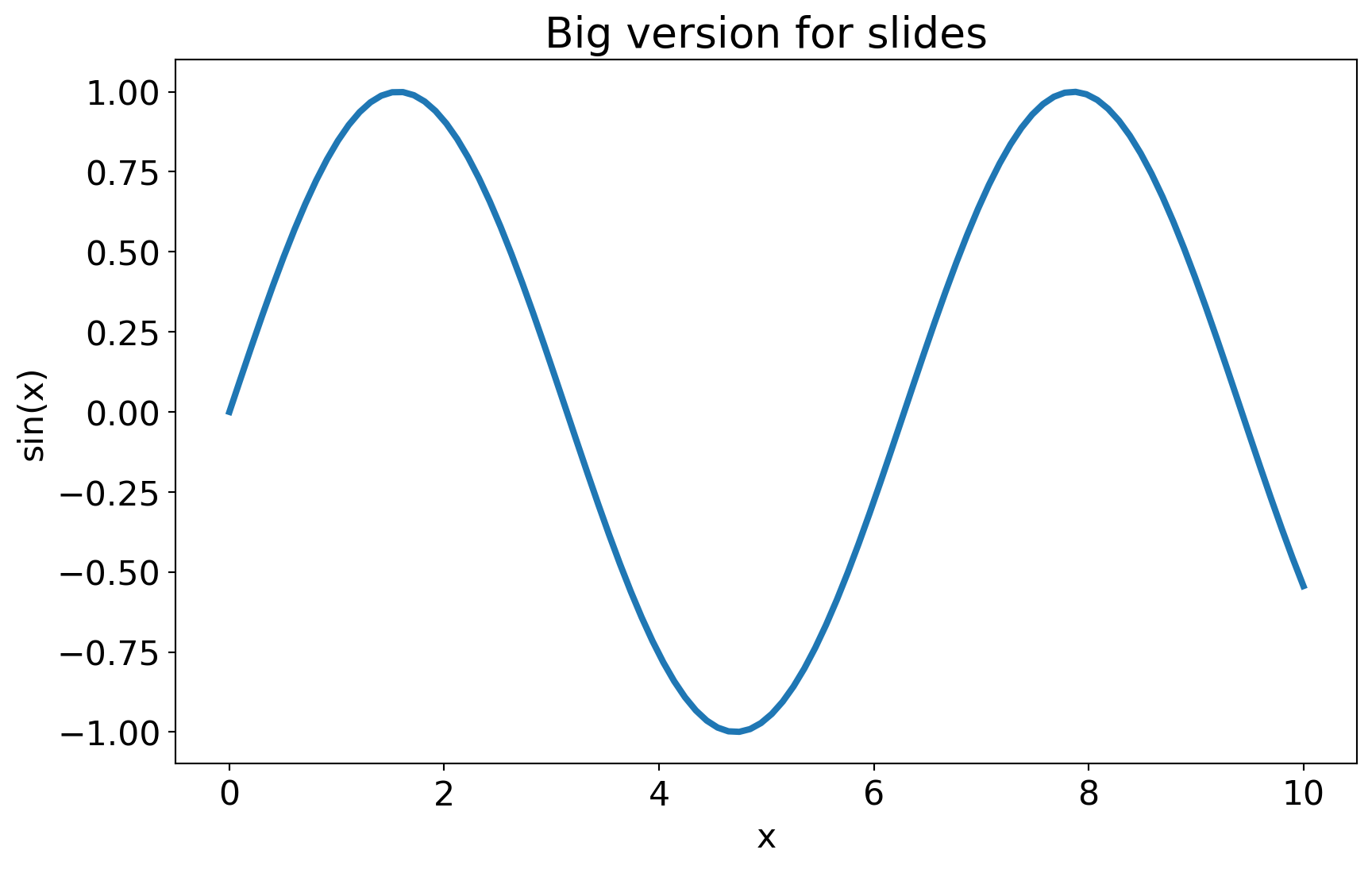

plt.rc_context() is the rcParams equivalent of plt.style.context(). Use a dictionary for ad-hoc tweaks and a style sheet for systematic styling.

8.8 8. ggplot2 → matplotlib styling cheat sheet

ggplot2	matplotlib
theme_minimal()	plt.style.use("seaborn-v0_8-whitegrid")
theme_bw()	plt.style.use("seaborn-v0_8-white")
theme_set(theme_minimal())	plt.style.use("...") for the session
theme(text = element_text(size = 12))	plt.rcParams["font.size"] = 12
theme(axis.text.x = element_text(angle = 45))	plt.rcParams["xtick.labelrotation"] = 45
theme(legend.position = "none")	no exact global equivalent; often control per-axes
custom theme function in R	custom .mplstyle file

The biggest conceptual difference: ggplot2 themes are functions that can be composed. Matplotlib styles are flat key-value files. They are less expressive but very easy to share.

8.9 9. Practical workflow recommendation

For radiology AI work, Quarto technical docs, and publication figures, a practical workflow is:

┌──────────────────────────────────────────────────────────┐
│ 1. One project-local style file: styles/radai.mplstyle   │
│    → captures fonts, palette, spine treatment, sizes     │
│                                                          │
│ 2. At the top of every notebook / script:                │
│    plt.style.use("styles/radai.mplstyle")                │
│                                                          │
│ 3. For a different output context, such as slides,       │
│    create radai-slides.mplstyle and use it instead.      │
│                                                          │
│ 4. For one-off tweaks, use plt.rc_context().             │
└──────────────────────────────────────────────────────────┘

Two style sheets can cover most cases:

• radai-paper.mplstyle: smaller figure and font sizes for journal columns
• radai-slides.mplstyle: larger figure and font sizes for projection

Same color palette, same spine treatment, different sizing.

8.10 10. Complete example: before and after

The same plotting function can produce different appearances depending only on the active style.

rng = np.random.default_rng(0)
x = np.linspace(0, 10, 50)

def make_plot():
    fig, ax = plt.subplots()
    ax.plot(x, np.sin(x), label="Sensitivity")
    ax.plot(x, np.cos(x), label="Specificity")
    ax.set_title("Diagnostic performance")
    ax.set_xlabel("Threshold")
    ax.set_ylabel("Performance")
    ax.legend()
    plt.show()

# Plot 1: factory defaults
with plt.style.context("default"):
    make_plot()

# Plot 2: project style
with plt.style.context("styles/radai.mplstyle"):
    make_plot()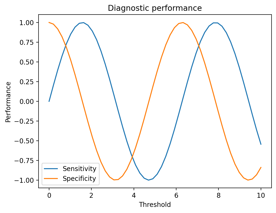

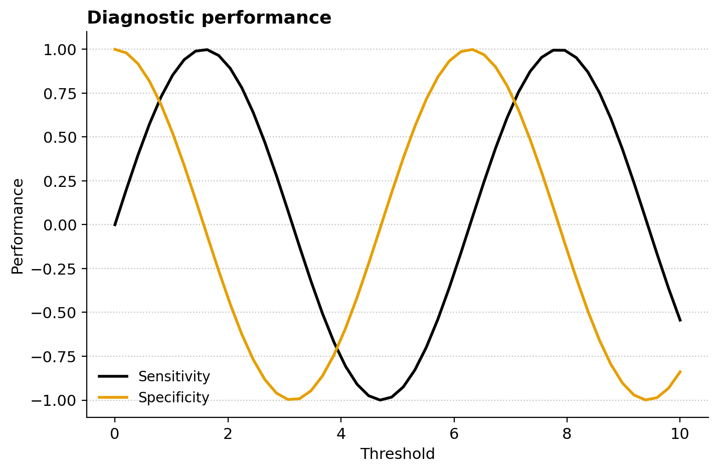
The function body is identical. The visual difference comes from the style. That is the payoff of this module.

8.11 Exercises

8.11.1 Exercise 1

In a fresh notebook, set these values with plt.rcParams.update(...), then make any simple line plot. Note which changes have visible effects.

plt.rcParams.update({
    "figure.figsize": (7, 4.5),
    "axes.titlesize": 14,
    "axes.titleweight": "bold",
    "axes.spines.top": False,
    "axes.spines.right": False,
    "axes.grid": True,
    "axes.grid.axis": "y",
    "grid.linestyle": ":",
    "grid.alpha": 0.4,
})

8.11.2 Exercise 2

Cycle through three built-in styles with plt.style.context(...):

• "ggplot"
• "seaborn-v0_8-whitegrid"
• "fivethirtyeight"

Draw the same plot in each. Note which feels closest to radiology publication style.

8.11.3 Exercise 3

Create radai.mplstyle with the contents from section 5, or your own variation. Save it next to the notebook or under a project styles/ folder. Apply it with:

plt.style.use("styles/radai.mplstyle")

Verify that a plot reflects the settings: Okabe-Ito colors, hidden top/right spines, and dotted y-grid.

8.11.4 Exercise 4

Create a second style file, radai-slides.mplstyle, identical to radai.mplstyle except:

figure.figsize: 11, 6.5
font.size: 16
axes.titlesize: 20
lines.linewidth: 3

Make the same plot with each style applied and compare.

8.11.5 Exercise 5: synthesis

Take the radiology dashboard from Module 6. Strip out the per-plot styling commands:

• no ax.spines[...].set_visible(...)
• no manual color hex codes
• no manual font sizes

Then apply the radai style at the top. The dashboard should still look polished, driven by the style file rather than inline styling.

This exercise shows the value of project-level styling most clearly.

8.12 Key takeaways

• rcParams is the central dictionary of matplotlib defaults.
• Per-plot keyword arguments are local; rcParams are session-wide; style sheets are reusable.
• plt.style.context(...) and plt.rc_context(...) are safer than global changes inside notebooks.
• A project-local .mplstyle file is best for Quarto books and reproducible publication workflows.
• Styling becomes powerful when plot code focuses on data while style files handle visual defaults.